Course progress Course outline 48 of 48 lessons available
Part 0 — Reading Guide: What Exactly Are We Going to Learn?
Part 1 — World Models: An Internal Sandbox for the Agent
Part 2 — Turning Images into State: The LeWM Architecture
- 06 Chapter 5 — Trajectory Data: To the Model, the World Is Not an Image Collection available now
- 07 Chapter 6 — The Visual Encoder: Issuing a “State Passport” for Every Frame available now
- 08 Chapter 7 — The Dynamics Predictor: Moving Time Forward in the Mind available now
- 09 Chapter 8 — A Complete Forward Pass: Follow One Batch from Start to Finish Current lesson
Part 3 — Preventing the Model from Cheating: Prediction Loss and SIGReg
- 10 Chapter 9 — The Most Dangerous Shortcut: Representation Collapse available now
- 11 Chapter 10 — Prediction Loss: How the Model Learns the Next Step available now
- 12 Chapter 11 — The Intuition Behind SIGReg: Letting Representation Space “Breathe” available now
- 13 Chapter 12 — Keep the Mathematics Minimal but Sufficient available now
- 14 Chapter 13 — The Original LeWM’s End-to-End Training Mechanism available now
- 15 Chapter 14 — Train a Model That Does Not Collapse Immediately available now
Part 4 — Putting the Model into Action: Planning in Latent Space
- 16 Chapter 15 — Goal-Conditioned Planning: From “Where Am I?” to “Where Do I Want to Go?” available now
- 17 Chapter 16 — Latent Euclidean Distance: Convenient, but Not Necessarily Reliable available now
- 18 Chapter 17 — CEM: Searching for Actions Through an Elimination Tournament available now
- 19 Chapter 18 — MPC: Do Not Trust the Model for Too Long at Once available now
- 20 Chapter 19 — Long-Horizon Rollouts: How Small Errors Snowball into Major Failures available now
- 21 Chapter 20 — Implement a Minimal LeWM Planner from Scratch available now
Part 5 — Engineering Reproduction: From Paper to Running System
- 22 Chapter 21 — The Official Repository and Experimental Environment available now
- 23 Chapter 22 — First Experiment: A TwoRoom Smoke Test available now
- 24 Chapter 23 — Second Experiment: Reproducing PushT available now
- 25 Chapter 24 — How to Evaluate a World Model Fairly available now
- 26 Chapter 25 — Failure-Diagnosis Manual available now
Part 6 — What Has LeWM Actually Learned?
- 27 Chapter 26 — Linear Probes: Which Physical Variables Are Encoded in the Latent State? available now
- 28 Chapter 27 — Give Latent Space a “Health Check” available now
- 29 Chapter 28 — Violation of Expectation: Is the Model Surprised by “Impossible Events”? available now
- 30 Chapter 29 — How to Discuss “Understanding the World” Rigorously available now
Part 7 — Why “Accurate Prediction” Can Still Produce “Poor Planning”
- 31 Chapter 30 — The Gap Between the Training Objective and the Planning Objective available now
- 32 Chapter 31 — Global Non-Collapse Does Not Guarantee Preservation of Task-Relevant Dynamics available now
- 33 Chapter 32 — When Is an Isotropic Gaussian Prior Too Strong? available now
- 34 Chapter 33 — Long-Horizon Planning: Predict Farther or Plan More Intelligently? available now
- 35 Chapter 34 — From Positional Distance to Task Progress available now
- 36 Chapter 35 — Multi-Task Learning, Real Robots, and Visual Distractions available now
- 37 Chapter 36 — Theoretical Boundaries: When Can the True State Be Identified? available now
Part 8 — From Reproducer to Researcher
Appendices
- 41 Appendix A — The Minimum Necessary Mathematical Toolkit available now
- 42 Appendix B — PyTorch Implementation Quick Reference available now
- 43 Appendix C — Complete Tensor-Shape Table available now
- 44 Appendix D — Experiment Configuration Cards available now
- 45 Appendix E — Paper Timeline and Evidence Levels available now
- 46 Appendix F — Glossary available now
- 47 Appendix G — Reproduction Checklist available now
- 48 Appendix H — Expert-Review Checklist available now
The big picture
- Encode fourz0 z1 z2 z3
- Align threea0 a1 a2
- Predict threep1 p2 p3
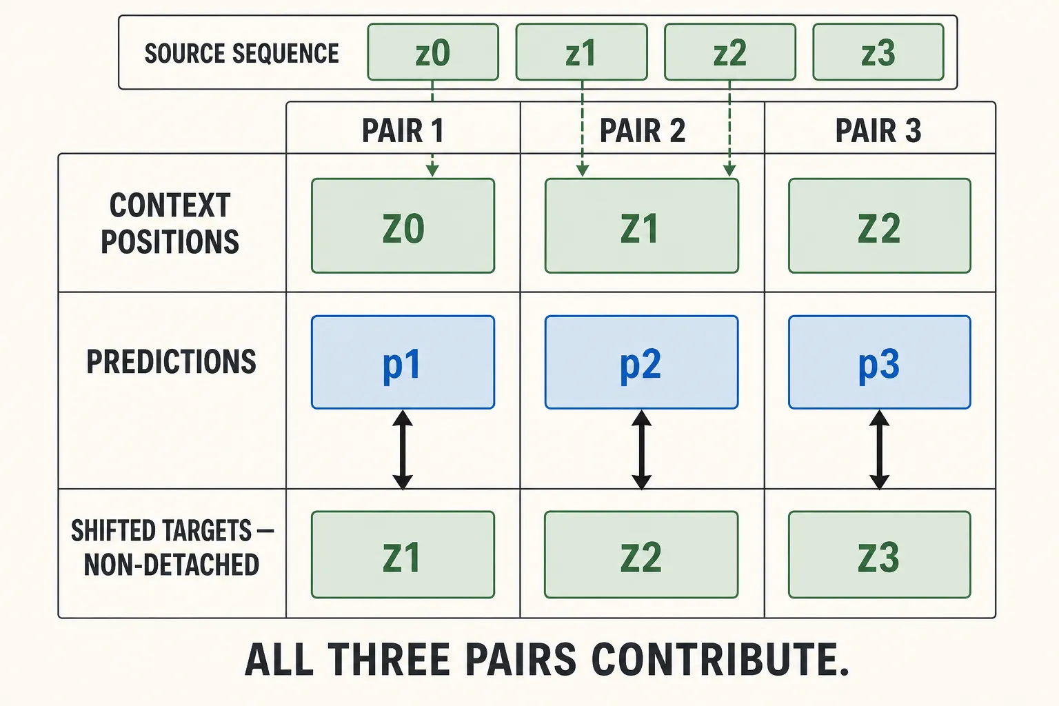
- Zip targetsp1↔z1, p2↔z2, p3↔z3
A tiny story
A factory can produce boxes of the right size with the wrong labels inside. A LeWM batch can do the same. Three predictions and three targets may match in shape even if each prediction is compared with the present instead of the next state, only the final pair is trained, or the target was detached.
This chapter’s simple promise is provenance: we can point to the observation, action block, prediction, and target at every slot.
The technical backpack
Frozen defaults make the whole forward pass concrete: batch B=128, history_size=3, num_preds=1, latent width D=192, and frameskip=5.
pixels                 [B,4,C,H,W]
flattened pixels       [B×4,C,H,W]
observation latents    [B,4,192]
raw action blocks      [B,4,5×A]
encoded actions        [B,4,192]
state/action context   [B,3,192]
connected targets      [B,3,192]
predictions            [B,3,192]
SIGReg input           [4,B,192]
losses                 scalar
The paper reports history one for TwoRoom and three for PushT/OGBench-Cube; the frozen global default is three. These shapes describe the frozen default, not every LeWM.
The shortest faithful forward card is:
z = encode_each_frame(images)              # [B,4,D]
u = encode_each_action_block(actions)       # [B,4,D]
z_pred = causal_predict(z[:,:3], u[:,:3])  # [B,3,D]
z_next = z[:,1:]                            # [B,3,D], do not detach
L_pred = mean_square_gap(z_pred, z_next)
L_sig = sigreg(time_first(z))               # [4,B,D]
L_total = L_pred + lambda * L_sig
All three shifted one-step pairs contribute. num_preds=1 means a one-position target offset, not one final output. A model step spans five environment actions in these data configs.
The prediction branch directly trains the visual encoder, encoder projector, action encoder, causal predictor, and prediction projector. Because z_next stays connected, prediction also returns through the target use of the same visual encoder. SIGReg directly trains only the visual encoder and its projector. One optimizer updates the connected learned system; there is no target-encoder optimizer or EMA update.
SIGReg sees each relative time position across the batch. It must not flatten B×T into one population, because temporal change is not the same as across-example diversity. Frozen code uses 1,024 random projections and 17 frequency knots from 0 through 3. The paper appendix presents quadrature differently. The paper method weight is 0.1; frozen YAML is 0.09. Keep every source label.
The trick that fools us
Make a deliberately wrong branch:
wrong targets: [z0,z1,z2]
right targets: [z1,z2,z3]
Both are [B,3,D]. The wrong branch can learn to copy the present and report a pleasing loss. Use visible time checksums and print prediction_slot / last_visible_context / target_source. Correct rows are 0/0/1, 1/1/2, 2/2/3.
Then test the graph. Detach only the correct target slice in a disposable probe and confirm that the target-side gradient route disappears while the context route remains. Merely finding some encoder gradient is not enough.
Five cheap checks catch most plumbing errors: exact shapes, shift provenance, causal future-mutation, finite/non-null gradients in every expected module, and no NaN or infinity. Passing them proves mechanics—not useful dynamics or planning.
Evidence receipt
LeWorldModel v3, frozen train.py, jepa.py, and module.py support the frozen alignment and connected graph. The paper’s displayed training pseudocode has a malformed F.mse_loss call, so executable train.py is the authority for exact indexing.
Do not call the next target a planning goal, detach it by JEPA habit, mix batch and time in SIGReg, or treat matching shapes as correctness.
Quick check
- Which three prediction–target pairs come from four observations?
- Through which two visual-encoder uses can prediction loss flow?
- Why can a wrong temporal target pass every ordinary shape assertion?