Chapter 6 — The Visual Encoder: Issuing a “State Passport” for Every Frame

The big picture

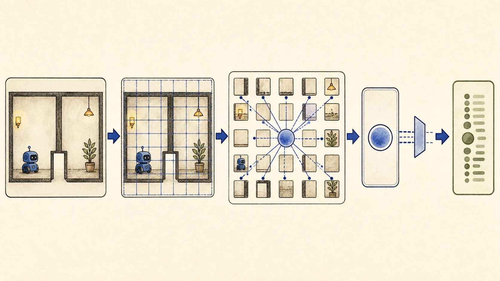
A tiny story

A camera frame is too large to carry through hundreds of imagined action plans. LeWM therefore gives each frame a small “state passport.” The predictor can move this passport through time much more cheaply than repainting the whole scene.

A real passport works because people agreed which fields matter. LeWM receives no such list. Its training pressures decide what survives. It may keep the doorway, or keep an easy wall color that merely correlates with the doorway.

The technical backpack

The frozen entry point first applies ImageNet-statistics preprocessing and resizes to 224×224. The default ViT-Tiny divides the image into 14×14 patches. Because 224 / 14 = 16, there are 16×16 = 256 patch tokens. Add one learned [CLS] token and the sequence length becomes 257.

The default backbone has width 192, 12 Transformer layers, and 3 attention heads. Attention lets spatial pieces exchange information. A patch is not an independently recognized object, and [CLS] is not magically semantic; it becomes useful only through the objective.

The visual encoder handles frames independently. It flattens batch and time, processes B×T images with shared weights, and then restores time. Temporal reasoning belongs to the later dynamics predictor.

[B,T,3,224,224]
  -> [B×T,3,224,224]
  -> [B×T,257,192]
  -> take [CLS]: [B×T,192]
  -> projector: [B×T,192]
  -> restore time: [B,T,192]

The projector is not a simple dimension reducer. Frozen code maps 192 → 2048 → 192 with BatchNorm and GELU between linear layers. The paper’s “1-layer MLP” and the code’s two linear maps are safely described as a one-hidden-layer projection MLP. Its output is the latent used by prediction and SIGReg.

LayerNorm normalizes features within one token. Projector BatchNorm uses statistics across flattened batch-time examples for each feature. SIGReg is a separate population loss. “Normalization makes it Gaussian” wrongly merges three mechanisms.

Original v3 sets pretrained: false: ViT, projector, action path, and dynamics learn together from offline trajectories.

The trick that fools us

Suppose wall color perfectly predicts which door is open in training. The encoder can store the color and ignore the tiny door gap. Repaint the wall without moving the door, and the passport changes too much. Move the door while keeping the color, and it changes too little.

Test three controlled pairs: vary texture with fixed geometry; vary geometry with matched texture; and swap only the nuisance while the frozen planner runs. A compact code, nonzero variance, or a good reconstruction does not prove the correct fact was retained.

Mechanical assertions still matter. Do not turn time into channels, forget to restore the time axis, or pass patch-level output where one state per frame is expected. Shapes can reveal a wrong implementation, though never a good representation by themselves.

Evidence receipt

LeWorldModel v3, frozen jepa.py, model configuration, and the frozen projection module support the exact default path. The paper also reports a ResNet-18 ablation, so ViT-Tiny is a baseline choice, not LeWM’s definition.

Allowed claim: [CLS] plus the projector is the latent carrier optimized by LeWM. Do not call it a complete world state, say BatchNorm imposes SIGReg’s Gaussian target, or infer physics from compactness.

Quick check

1. Why do 224-pixel sides and patch size 14 produce 256 patches?
2. Which component handles time after frames are encoded independently?
3. How would you expose a passport that follows wall color instead of doorway geometry?