Chapter 9 — The Most Dangerous Shortcut: Representation Collapse

The big picture

A tiny story

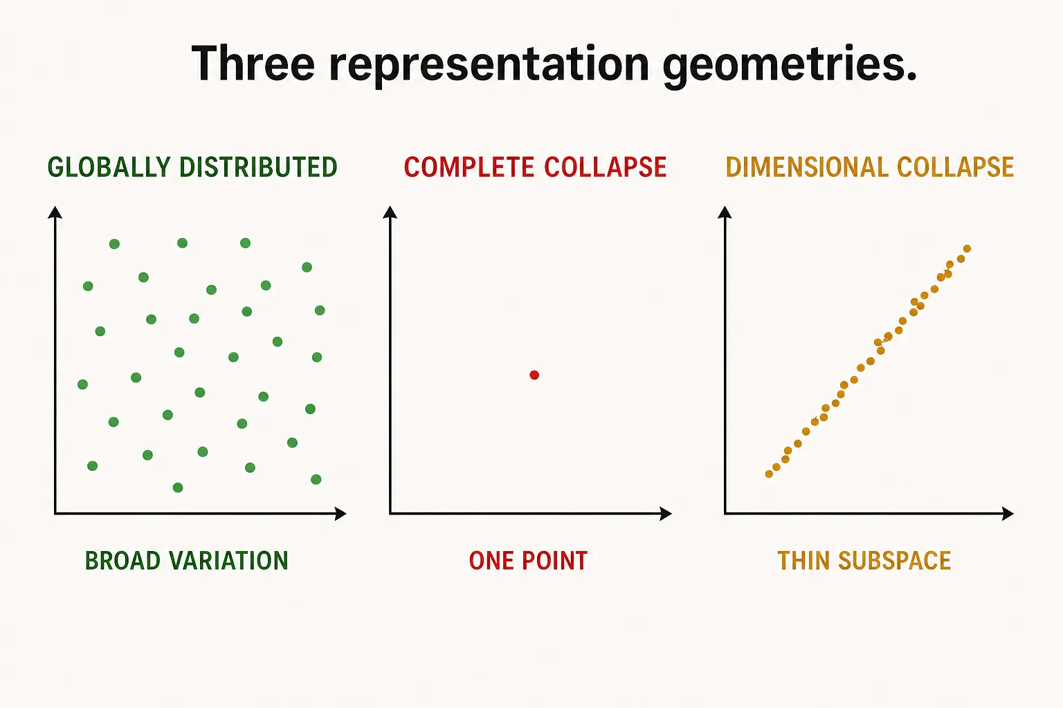
Imagine a passport office that stamps every traveler with the same card. Its records are wonderfully consistent: every “next passport” matches every prediction. They are useless for telling anyone apart.

That is complete representation collapse. Dimensional collapse is subtler: passports vary, but almost all information lies on one thin road inside a much larger latent space. Low intrinsic dimension can also be legitimate, so thinness is a warning relative to the data and task—not an automatic verdict.

The real rule

The loophole fits in four lines:

encode(any_image) -> the_same_vector
predict(any_vector, any_action) -> the_same_vector
prediction_gap -> zero
state distinctions -> gone

It works because the next target is produced by the same trainable encoder. It is not a fixed physical answer key. Prediction-only training therefore admits the constant solution; that does not mean every low-loss run finds it.

SIGReg adds a population-shape target. One repeated point cannot match a non-degenerate isotropic standard Gaussian, so the exact constant shortcut conflicts with the ideal joint objective. That claim is deliberately narrow. A broad cloud can encode background color, ignore action, or arrange states in a geometry that misleads planning.

Collapse is also not overfitting. A model can collapse on both train and validation data, or preserve rich training distinctions yet generalize badly. Measure both representation structure and held-out behavior.

Useful screens work together:

• per-coordinate variance for obvious contraction;
• covariance spectrum for rotated thin subspaces;
• effective rank for comparing matched runs;
• pairwise-distance distributions and duplicate rates;
• nearest-neighbor panels tied back to observations;
• action-swap sensitivity for control use.

None is proof. Identity-like covariance captures only second-order structure. Full rank does not prove dynamics. Attractive neighbors can follow color rather than reachability.

The trick that fools us

Train matched tiny TwoRoom runs with and without SIGReg. At every checkpoint, keep the same probe batch and record prediction loss, raw SIGReg, variance, covariance spectrum, effective rank, pairwise distances, neighbors, and action swaps.

The hypothesis is not “the no-SIGReg run must collapse.” It is: removing the population term restores a trivial optimum that prediction alone cannot reject. If the cloud remains broad, complete collapse was avoided, but action and rollout tests are still required. If a diverse input batch becomes a thin latent cloud, the evidence is stronger than a rank number from one narrow room corner.

Evidence receipt

LeWorldModel v3 identifies the constant shortcut and uses SIGReg. LeJEPA v3 motivates complete versus dimensional collapse and the hidden-X example showing why simple axis checks can miss dependence. Frozen train.py logs prediction, SIGReg, and total separately.

The single-seed independent TwoRoom report measured position-probe Pearson correlation 0.9988, close to the paper’s 0.996. That says position was linearly accessible in that representation. It does not prove SIGReg caused the result, the predictor used position, or the representation learned physics.

Quick check

1. Why can constant codes produce perfect next-latent agreement?
2. How is dimensional collapse different from overfitting?
3. Why must several latent diagnostics agree before you diagnose collapse?