Appendix C — Complete Tensor-Shape Table

Trace tensors from [B,T,C,H,W] through [B,T,D] to [B,N,H,D], including dimension meanings, broadcasting rules, and common errors.

Course progress Course outline 48 of 48 lessons available

Part 0 — Reading Guide: What Exactly Are We Going to Learn?

01 Chapter 0 — Before You Begin available now

Part 1 — World Models: An Internal Sandbox for the Agent

Part 2 — Turning Images into State: The LeWM Architecture

06 Chapter 5 — Trajectory Data: To the Model, the World Is Not an Image Collection available now
07 Chapter 6 — The Visual Encoder: Issuing a “State Passport” for Every Frame available now
08 Chapter 7 — The Dynamics Predictor: Moving Time Forward in the Mind available now
09 Chapter 8 — A Complete Forward Pass: Follow One Batch from Start to Finish available now

Part 3 — Preventing the Model from Cheating: Prediction Loss and SIGReg

Part 4 — Putting the Model into Action: Planning in Latent Space

Part 5 — Engineering Reproduction: From Paper to Running System

Part 6 — What Has LeWM Actually Learned?

Part 7 — Why “Accurate Prediction” Can Still Produce “Poor Planning”

Part 8 — From Reproducer to Researcher

Appendices

The big picture

Real frames[B,T,C,H,W]
Latent journey[B,T,D]
Shift one stepcontext → next target
Many futures[B,N,H,D]

A shape says how many seats exist. Axis names say who sits in them.

Frames pass through one shared per-frame encoder and return as a latent journey.

A tiny story

Two suitcases can have identical dimensions and belong on different flights. Tensors are the same. A reshape can preserve every value while turning time into candidate identity. A broadcast can produce the expected shape while copying a goal along the wrong axis. The program runs; the story is broken.

Use these names every time: B batch, T recorded observation position, C channel, image H/W spatial size, D latent width, N candidate sequence, planning H model horizon, U control-block width, F environment ticks per model step, A action width, P image patches, and Dv internal vision width. The two meanings of H are a notation hazard: say image height or planning horizon.

The shape backpack

Lane 1: observations become state cards

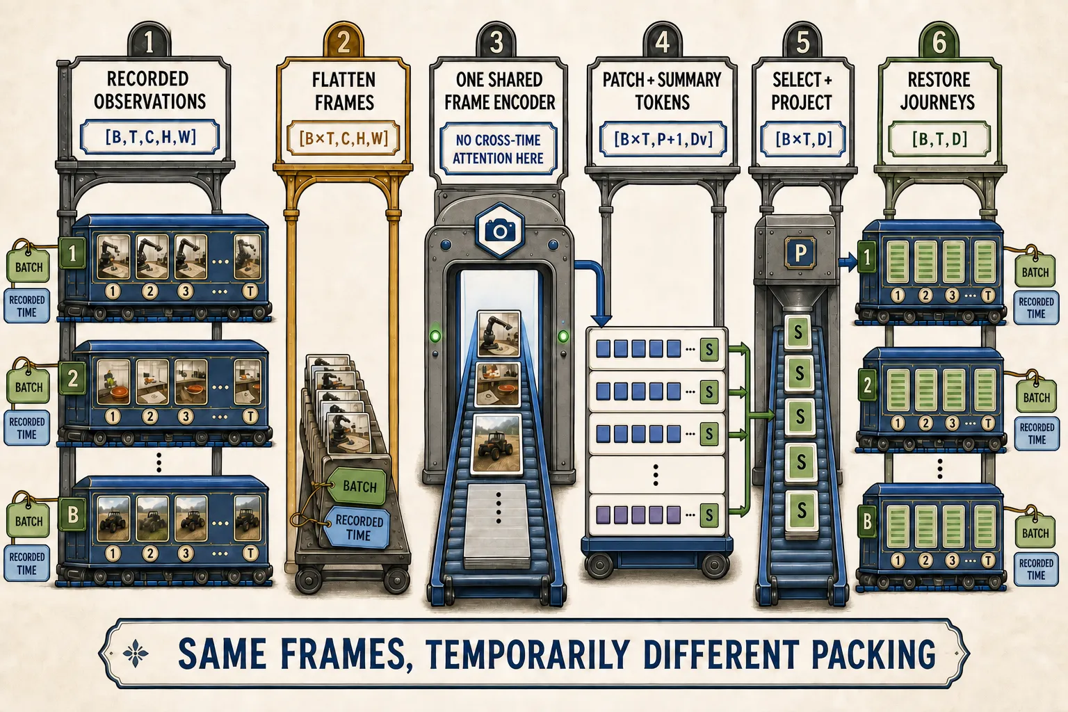
The visual encoder handles frames independently. It temporarily folds batch and recorded time into a frame batch, encodes each image, selects the summary token, projects it, and restores the journey.

Stop	Shape	Meaning	Silent danger
loaded observations	`[B,T,C,H,W]`	example, recorded time, channel, image height, image width	shuffle frames inside a journey
frame batch	`[B×T,C,H,W]`	independent frames, channel, height, width	restore `B` and `T` in the wrong order
ViT tokens	`[B×T,P+1,Dv]`	frame, patches plus summary, visual width	mistake patch order for episode time
projected frames	`[B×T,D]`	frame, latent feature	select the wrong token or layer
latent journey	`[B,T,D]`	example, recorded time, latent feature	silently swap batch and time

Flattening [B,T] does not give the visual encoder temporal attention; it only makes a larger independent frame batch. P, Dv, and D remain different roles even if two numeric values happen to match.

Lane 2: actions align with transitions

Actions do not enter as image channels. In the frozen baseline, F=5 consecutive environment actions form one model-step control block. The action encoder maps that block to width D.

Stop	Shape	Meaning	Silent danger
raw action blocks	`[B,T,F×A]`	example, model position, grouped controls	cross an episode boundary
encoded actions	`[B,T,D]`	example, model position, conditioning feature	shift the action one transition late
training action context	`[B,T-1,D]`	source transition positions	use the final loaded slot as an extra target

The loaded observations and actions may both have length T; the one-step objective still uses only the first T-1 source actions. Test alignment with distinctive actions, not all-zero controls that look unchanged after a shift.

Lane 3: the shifted zipper

With four encoded observations, the contract is:

z0 with a0 -> p1 compared with connected z1
z1 with a1 -> p2 compared with connected z2
z2 with a2 -> p3 compared with connected z3

Object	Shape	Role
state context	`[B,T-1,D]`	real encoded source positions
action context	`[B,T-1,D]`	actions aligned to those sources
predictor output	`[B,T-1,D]`	predicted successors
shifted target	`[B,T-1,D]`	real encoded successor positions
SIGReg view	`[T,B,D]`	each recorded time inspected across its batch population

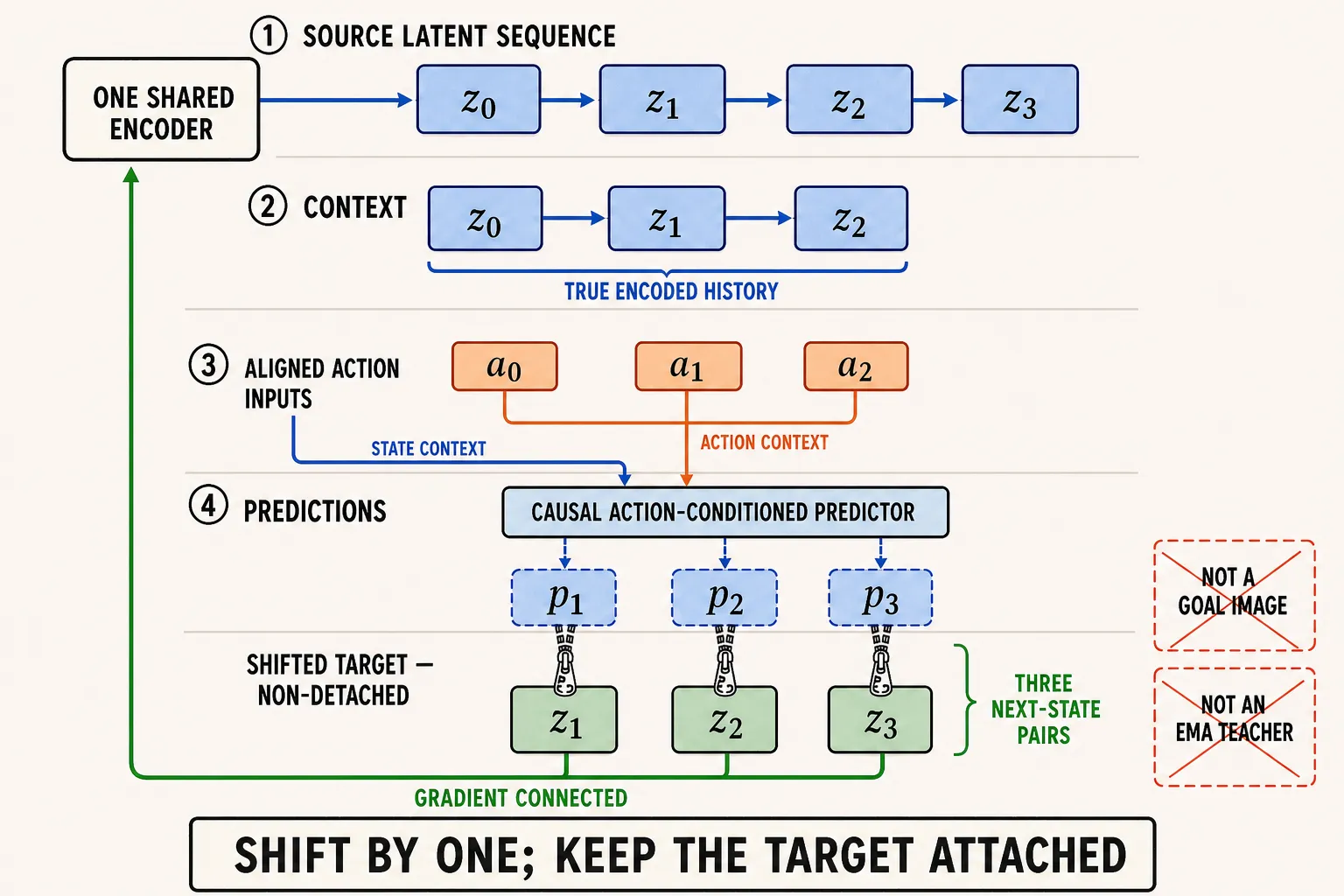
Three predictions zip to the next three connected encoder targets.

Prediction and target shapes matching is necessary, not sufficient: comparing p1,p2,p3 with z0,z1,z2 still returns a scalar and teaches the wrong relation. In original LeWM v3, z1,z2,z3 come from the same shared trainable encoder and remain connected—no stop-gradient, EMA teacher, or pretrained frozen encoder. Detaching them changes the graph without changing any shape. SIGReg also keeps time positions distinct; flattening T and B changes the population it measures.

Lane 4: planning opens candidate lanes

Planning has no real future frame for each hypothetical action. It repeats one observed current state across candidate lanes, then rolls the frozen predictor forward autoregressively.

Object	Shape	Role and allowed copy
current state	`[B,D]` or history-aware equivalent	repeat only across candidates
candidate actions	`[B,N,H,U]`	problem, candidate, model horizon, control block
predicted rollout	`[B,N,H,D]`	time stays sequential inside each candidate
encoded goal	`[B,D]`	repeat across candidate endpoints only
terminal endpoints	`[B,N,D]`	one predicted endpoint per candidate
candidate cost	`[B,N]`	preserve mapping back to action sequences

An implementation may flatten [B,N] for GPU execution, but it must restore candidate ownership. One environment’s low-cost route cannot select another environment’s action. The goal is copied across candidates because they share a destination; it is not copied across predictor time as training supervision.

Frozen numeric card—not a universal constant

The inspected code’s checked-in default uses batch 128, history size 3, therefore 4 loaded observation positions, latent width 192, one-step shifted targets, and 5 environment actions per model position. One concrete prediction/target shape is [128,3,192].

The paper reports history 1 for TwoRoom and 3 for PushT and OGBench-Cube, while the frozen global default is 3 and data configs do not override it. [B,T,D] is a symbolic contract; [128,4,192] is one frozen-code instance. Always label paper, frozen code, and resolved run separately.

The trick that fools us

A dashboard says images are 5-D, prediction and target are [128,3,192], candidate cost is [1,1024], and total loss is scalar. Every light is green. Yet the target is unshifted, candidate and horizon axes were swapped when both had length five, and the goal was copied across time instead of candidates.

Repair this with a tiny marked batch: two episode IDs, distinct time marks, distinct candidate IDs, and non-repeating actions. Then perturb one later token, one candidate action, and one goal. Earlier causal outputs should ignore the later token; only that candidate lane should react to its action; changing the goal should change costs, not model rollouts. These checks prove plumbing invariants, not model accuracy.

Evidence receipt

LeWorldModel v3 and frozen official train.py, jepa.py, module.py, and configuration files support the cited routes and frozen defaults.

Allowed claim: a faithful implementation preserves named observation, time, action, candidate, horizon, target, and latent roles even when storage is rearranged. A passing shape assertion does not prove alignment, broadcasting, gradient flow, planning semantics, or paper reproduction. Independent reproduction is not established here.

Quick check

Why does [B×T,C,H,W] not create temporal attention by itself?
Which targets belong with p1,p2,p3, and why can the wrong targets pass a shape check?
In [B,N,H,D], which axis can run in parallel and which dependence remains sequential?