Chapter 11 — The Intuition Behind SIGReg: Letting Representation Space “Breathe”

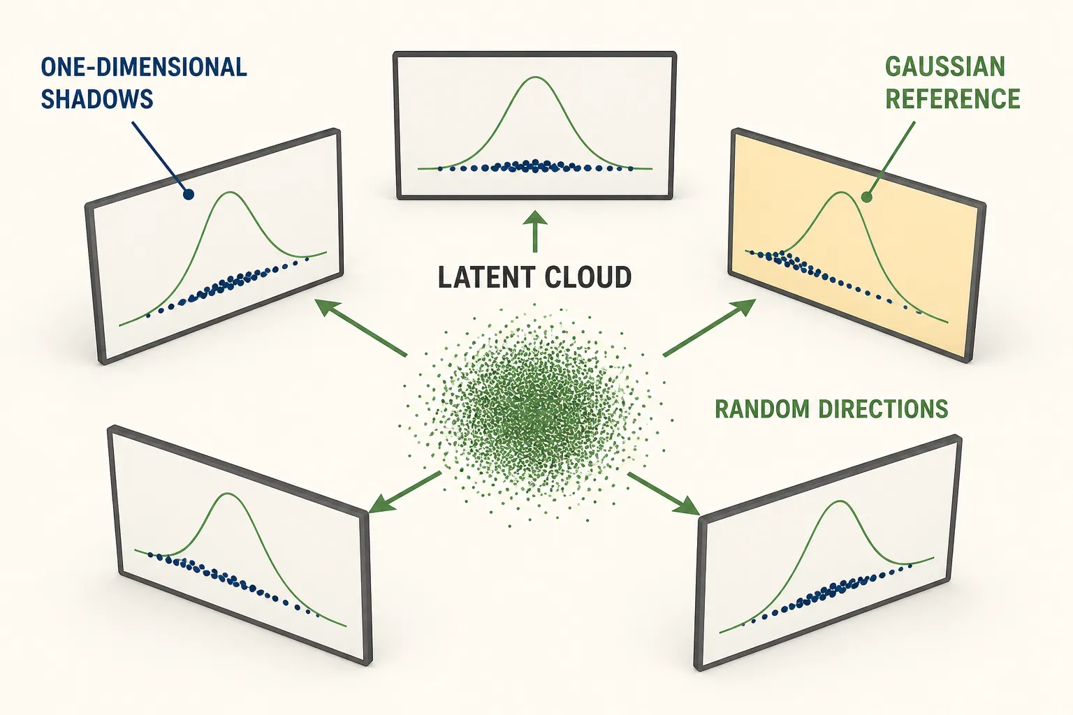
The big picture

A tiny story

“Do not put everyone at one address” is too vague. A city can avoid one point yet squeeze every resident onto one road, stretch into one dominant direction, or make an X-shaped pattern whose simple statistics look healthy.

SIGReg—Sketched Isotropic Gaussian Regularization—gives the crowd a reference shape. It asks many one-dimensional shadows of the embedding population to resemble shadows from an isotropic standard Gaussian.

The technical backpack

At each relative time position, frozen LeWM treats the B embeddings as one population. Time is not mixed into the crowd. A random unit vector turns every D=192 embedding into one signed scalar shadow. Repeat across directions and compare each one-dimensional sample with the analytic Gaussian fingerprint.

The Gaussian words matter:

• standard: each unit-direction shadow is centered at zero with unit scale;
• isotropic: the reference has no preferred direction;
• Gaussian: it is not a uniform ball. Density peaks at the origin, while high-dimensional radial probability mass concentrates roughly near radius sqrt(D).

The Epps–Pulley construction uses an empirical characteristic function. At finite frequency probes, it averages cosine and sine responses and compares them with the known standard-Gaussian responses. LeWM minimizes a smooth discrepancy; it does not compute a p-value or declare that a batch “passed normality.”

[T,B,D]
  -> for each time: B-point cloud
  -> random 1D projections
  -> cosine/sine responses at finite knots
  -> gap to analytic N(0,1) fingerprint
  -> average across directions and time

Frozen code samples 1,024 directions per call and uses 17 knots from 0 through 3 with a Gaussian weighting window. Directions are resampled, so the training value is stochastic. The class is marked single-GPU and does not gather a global population across devices. The paper appendix presents an illustrative integration differently; keep paper and executable facts separate.

The Cramér–Wold principle identifies multivariate distributions if all one-dimensional projections match. Frozen training sees finite batches, finite directions, and finite knots. It is an approximation, not a Gaussianity certificate.

The trick that fools us

Inspect only horizontal and vertical axes of an X-shaped cloud. Both shadows can look harmless while a diagonal shadow reveals dependence. Random views reduce permanent blind spots, but 1,024 finite views can still miss a narrow defect.

Now inspect a real corridor trajectory. A thin cloud may reflect a genuinely low-dimensional world rather than a broken encoder. Forcing it into a 192-dimensional isotropic target can create tension. The LeWM paper suggests this mismatch as a possible contributor in TwoRoom; it is an author hypothesis, not an established cause.

More projections do not create more observations. Looking at a small crowd from a thousand angles does not make it a large crowd. Batch size and projection count address different uncertainty.

Evidence receipt

The mechanism comes from LeWorldModel v3, frozen SIGReg, LeJEPA v3, the Epps–Pulley paper, and Cramér–Wold.

SIGReg needs batch examples but no labelled negatives and no learned teacher because its reference is analytic. Matching that reference excludes the exact constant representation at the ideal target. It does not prove physics, action sensitivity, reachability, or finite-run success.

Quick check

1. Why are nonzero variance and identity covariance still incomplete checks?
2. Why do finite random projections not turn Cramér–Wold into a proof?
3. What does SIGReg use instead of negative pairs or an EMA teacher?