Course progress Course outline 48 of 48 lessons available
Part 0 — Reading Guide: What Exactly Are We Going to Learn?
Part 1 — World Models: An Internal Sandbox for the Agent
Part 2 — Turning Images into State: The LeWM Architecture
- 06 Chapter 5 — Trajectory Data: To the Model, the World Is Not an Image Collection available now
- 07 Chapter 6 — The Visual Encoder: Issuing a “State Passport” for Every Frame available now
- 08 Chapter 7 — The Dynamics Predictor: Moving Time Forward in the Mind available now
- 09 Chapter 8 — A Complete Forward Pass: Follow One Batch from Start to Finish available now
Part 3 — Preventing the Model from Cheating: Prediction Loss and SIGReg
- 10 Chapter 9 — The Most Dangerous Shortcut: Representation Collapse available now
- 11 Chapter 10 — Prediction Loss: How the Model Learns the Next Step available now
- 12 Chapter 11 — The Intuition Behind SIGReg: Letting Representation Space “Breathe” available now
- 13 Chapter 12 — Keep the Mathematics Minimal but Sufficient available now
- 14 Chapter 13 — The Original LeWM’s End-to-End Training Mechanism available now
- 15 Chapter 14 — Train a Model That Does Not Collapse Immediately available now
Part 4 — Putting the Model into Action: Planning in Latent Space
- 16 Chapter 15 — Goal-Conditioned Planning: From “Where Am I?” to “Where Do I Want to Go?” available now
- 17 Chapter 16 — Latent Euclidean Distance: Convenient, but Not Necessarily Reliable available now
- 18 Chapter 17 — CEM: Searching for Actions Through an Elimination Tournament available now
- 19 Chapter 18 — MPC: Do Not Trust the Model for Too Long at Once available now
- 20 Chapter 19 — Long-Horizon Rollouts: How Small Errors Snowball into Major Failures available now
- 21 Chapter 20 — Implement a Minimal LeWM Planner from Scratch available now
Part 5 — Engineering Reproduction: From Paper to Running System
- 22 Chapter 21 — The Official Repository and Experimental Environment available now
- 23 Chapter 22 — First Experiment: A TwoRoom Smoke Test available now
- 24 Chapter 23 — Second Experiment: Reproducing PushT available now
- 25 Chapter 24 — How to Evaluate a World Model Fairly available now
- 26 Chapter 25 — Failure-Diagnosis Manual available now
Part 6 — What Has LeWM Actually Learned?
- 27 Chapter 26 — Linear Probes: Which Physical Variables Are Encoded in the Latent State? available now
- 28 Chapter 27 — Give Latent Space a “Health Check” available now
- 29 Chapter 28 — Violation of Expectation: Is the Model Surprised by “Impossible Events”? available now
- 30 Chapter 29 — How to Discuss “Understanding the World” Rigorously available now
Part 7 — Why “Accurate Prediction” Can Still Produce “Poor Planning”
- 31 Chapter 30 — The Gap Between the Training Objective and the Planning Objective available now
- 32 Chapter 31 — Global Non-Collapse Does Not Guarantee Preservation of Task-Relevant Dynamics available now
- 33 Chapter 32 — When Is an Isotropic Gaussian Prior Too Strong? available now
- 34 Chapter 33 — Long-Horizon Planning: Predict Farther or Plan More Intelligently? available now
- 35 Chapter 34 — From Positional Distance to Task Progress available now
- 36 Chapter 35 — Multi-Task Learning, Real Robots, and Visual Distractions available now
- 37 Chapter 36 — Theoretical Boundaries: When Can the True State Be Identified? available now
Part 8 — From Reproducer to Researcher
Appendices
- 41 Appendix A — The Minimum Necessary Mathematical Toolkit Current lesson
- 42 Appendix B — PyTorch Implementation Quick Reference available now
- 43 Appendix C — Complete Tensor-Shape Table available now
- 44 Appendix D — Experiment Configuration Cards available now
- 45 Appendix E — Paper Timeline and Evidence Levels available now
- 46 Appendix F — Glossary available now
- 47 Appendix G — Reproduction Checklist available now
- 48 Appendix H — Expert-Review Checklist available now
The big picture
- Name the axeswho, when, what?
- Inspect the cloudcenter, spread, shape
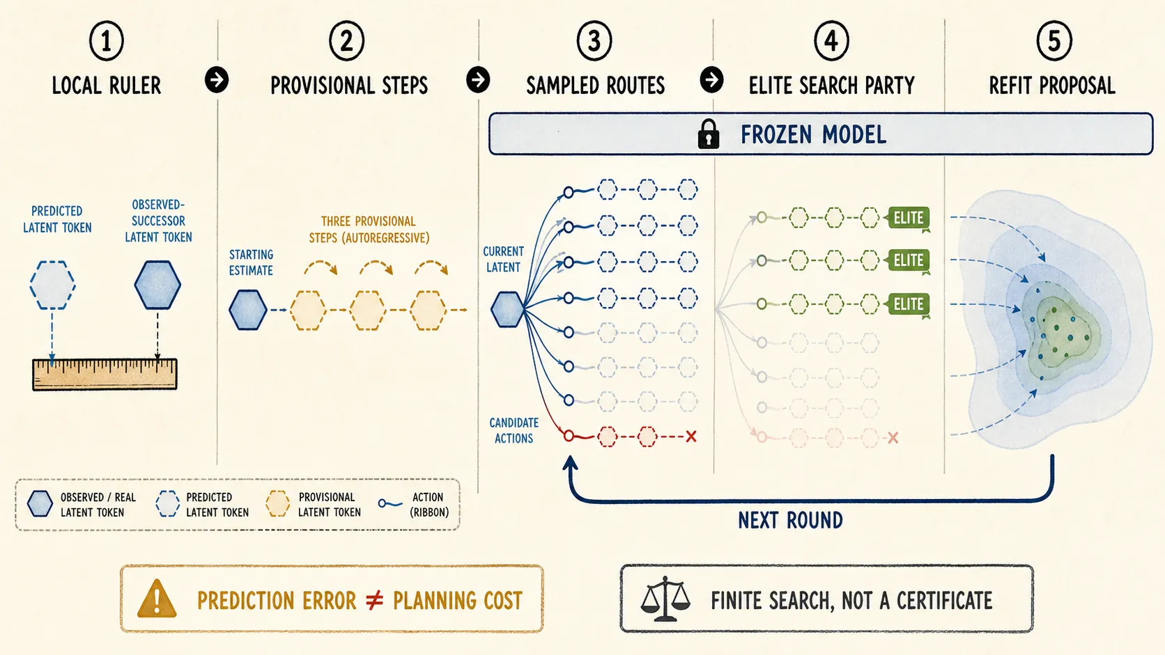
- Measure a misslocal ruler only
- Search futuressample, keep, narrow
A pocket story
Imagine a control room with ten instruments. One labels boxes. Three describe a crowd. One shines lights to see shadows. One traces who receives blame. One measures a miss. One watches errors step into the future. One asks sampled witnesses. The last sends a search party.
All ten can display green while the agent still chooses an impossible shortcut through a wall. That is the lesson of this appendix: a correct measurement can answer the wrong question. Before trusting a number, ask, “What job does this tool do, and what can it not know?”
The technical backpack
1. Labels before arithmetic
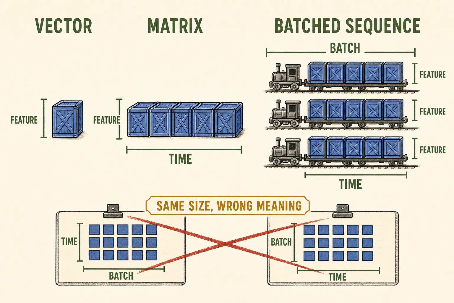
A vector is one state card; a matrix is a table of cards; a tensor adds more labelled axes. [B,T,D] means batch, recorded time, latent feature. During planning, [B,N,H,D] means environment batch, candidate, model horizon, latent feature. Two tensors can contain the same number of values and tell different stories after an axis swap. Say every axis aloud.
2. Three crowd summaries
For latent vectors z1 ... zn, the mean is the crowd’s center:
mean = (z1 + ... + zn) / nVariance measures spread along one coordinate. Covariance asks whether coordinates move together; its spectrum shows whether variation uses many directions or only a thin sheet. These are alarms, not meaning certificates. A feature can vary only because brightness varies, and two clouds can share mean and covariance while differing in holes, branches, or rare contact states.
SIGReg points the population toward an isotropic standard Gaussian: centered, broadly spread, and without a privileged direction. This excludes the exact one-code-for-everything collapse. It does not prove that doorway, position, or physics has useful coordinates. In high dimensions, density is highest at the origin while most radial mass lies in a broad shell; “Gaussian” does not mean “every point sits at zero.”
3. Shadows and gradients
A random projection turns a high-dimensional cloud into a one-dimensional shadow. The Cramér–Wold idea says that agreement in every direction identifies a distribution. Practical SIGReg sees only finite directions, a finite minibatch, and finite numerical integration. It is repeated pressure, not a Gaussianity certificate.
A gradient is a local trail of responsibility. In original LeWM v3, there is one shared trainable visual encoder. The next-observation target stays connected: no stop-gradient, EMA teacher, or pretrained frozen encoder is added. Prediction loss therefore reaches the predicted branch and the shifted target branch; SIGReg reaches projected observation embeddings. A path existing does not guarantee a strong, well-scaled, helpful signal. lambda only balances population-shape pressure against prediction pressure.
4. Rulers, stepping stones, and witnesses
Mean squared error compares matching coordinates and punishes larger coordinate gaps more strongly:
MSE = mean((predicted_next_latent - connected_next_latent)^2)It says the named vectors are close under this ruler. It does not say the latent is non-collapsed, actions matter, a rollout stays stable, or a goal is reachable. Squared terminal distance can rank two states across a wall as close even when the feasible route is long.
Teacher-forced one-step prediction stands on recorded observations. An autoregressive rollout places the next stepping stone on a model-generated stone. Errors may compound, cancel, saturate, or trigger a branch change near a doorway or contact boundary; there is no universal growth curve.
Monte Carlo estimation asks sampled witnesses when enumeration is too expensive. More appropriate independent samples can reduce sampling noise. They cannot repair model bias, missing data support, or a wrong cost.
5. CEM is the search party
start with a broad action proposal
repeat for a configured number of rounds:
    sample candidate action sequences
    imagine endpoints with the frozen world model
    rank endpoints with the configured cost
    refit the proposal toward the elite candidates
return the configured output (paper Appendix B prose: final proposal mean)
CEM changes the action proposal, not encoder or predictor weights. A candidate never sampled cannot become elite; a proposal can narrow too early; stronger search can exploit a model or cost flaw more effectively. Finite CEM is not a global-optimum certificate.
The trick that fools us
Suppose mean, variance, covariance, sampled shadows, and one-step MSE all look healthy. CEM also converges sharply. Now reveal that opposite sides of the TwoRoom wall are neighbors in latent space, so terminal distance rewards walking through the wall.
Nothing on the dashboard had to be computed incorrectly. Population statistics described global shape; MSE described recorded local transitions; CEM optimized the frozen model and chosen cost. None directly tested route reachability.
A useful experiment separates those questions. Keep a fixed set of doorway cases. Log population geometry, action swaps, one-step error, self-fed error by horizon, predicted route, cost ranking, and real execution. If more CEM samples only make the impossible shortcut win more reliably, investigate model support and cost geometry before enlarging the search again.
Evidence receipt
LeWorldModel v3 and the frozen official code at 8edfeb336732b5f3ce7b8b210d0ba370a09e2cac support the connected shared-encoder graph and planning roles. LeJEPA v3, the Epps–Pulley test, and the Cramér–Wold theorem support the assumption-bounded projection motivation.
Allowed claim: these tools describe tensor meaning, population summaries, local prediction gaps, stochastic estimates, and finite search under named assumptions. Not allowed: healthy statistics prove semantic state recovery; finite projections prove Gaussianity; low MSE proves reachability; more samples repair a wrong model; CEM proves a global optimum. Independent reproduction is not established here.
Quick check
- Why can a shape-preserving axis swap still break the system?
- Why can a Gaussian-looking latent cloud still forget the doorway?
- If CEM confidently selects an impossible route, which measurements would you separate next?